Hey there, it’s Anthony, ready to bring an end to this epic trilogy of identifying hazmat signs.
In this part we will cover how we solved the second half of the generic object detection problem (as detailed in the first part): classification.
The algorithms used in this part are by far the most complicated. Rather than a tutorial on how the algorithms work, this is better described as a tutorial on how to use OpenCV functions that execute the algorithms. Therefore, there will be a lot more code and less explanations than in the first two parts.
First, an algorithm called Scale-Invariant Feature Transform (SIFT) can be used to find “key points” in an image. When applied to a sample image of a hazmat sign, the following output can be found:
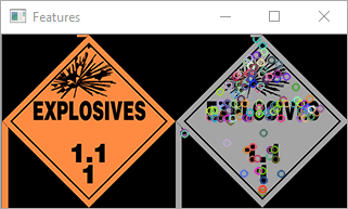
It should be noted that SIFT has detected text as features. This enabled us to forego implementing standalone text detection. SIFT has been accurate enough to tell the difference between signs whose only difference is text (like explosives 1.1 and 1.2) surprisingly consistently. The above output was generated by the following code:
1 2 3 4 5 6 7 8 9 10 11 12 13 14 15 16 17 18 19 20 21 22 23 24 25 26 27 28 29 30 31 32 33 34 35 36 37 38 | # imports import cv2, numpy # read the image img = cv2.imread('template.png') # make it grayscale gray = cv2.cvtColor(img.copy(), cv2.COLOR_BGR2GRAY) # make a new variable called 'out' as a copy of the input image out = img.copy() # make a new SIFT detector object as per the opencv implementation sift = cv2.xfeatures2d.SIFT_create() # store the key points of our SIFT detector's detections in the variable kp kp = sift.detect(gray, None) # draw them using opencv's keypoint drawing function onto the 'out' image defined above cv2.drawKeypoints(gray, kp, outImage=out) # append the first and second image together final = numpy.hstack((img, out)) # display the two images appended together cv2.imshow("Features", final) # await a key press cv2.waitKey(0) |
An algorithm called k-nearest-neighbors (KNN) can be used to match the similarity of two images based on their features, found by SIFT. The best matching features are chosen, appended to an array called ‘good’ and outputted, as in the following python function:
1 2 3 4 5 6 7 8 9 10 11 12 13 14 15 16 17 18 19 20 21 22 | def bff_match(image, template): # Initiate SIFT detector sift = cv2.xfeatures2d.SIFT_create() # find the keypoints and descriptors with SIFT kp1, des1 = sift.detectAndCompute(image, None) # apparently this only works with 8-bit images kp2, des2 = sift.detectAndCompute(template, None) FLANN_INDEX_KDTREE = 0 index_params = dict(algorithm = FLANN_INDEX_KDTREE, trees = 5) search_params = dict(checks = 50) flann = cv2.FlannBasedMatcher(index_params, search_params) matches = flann.knnMatch(des1, des2, k=2) # store all the good matches as per Lowe's ratio test. good = [] for m,n in matches: if m.distance < MIN_MATCH_RATING*n.distance: good.append(m) # return the number of matches (the tutorial describes how to draw the features if interested) return good |
By feeding the output of that function into the following code:
1 2 3 4 5 6 7 8 9 10 11 12 13 14 15 16 17 18 19 20 21 | if len(good)>MIN_MATCH_COUNT: src_pts = np.float32([ kp1[m.queryIdx].pt for m in good ]).reshape(-1,1,2) dst_pts = np.float32([ kp2[m.trainIdx].pt for m in good ]).reshape(-1,1,2) M, mask = cv2.findHomography(src_pts, dst_pts, cv2.RANSAC,5.0) matchesMask = mask.ravel().tolist() h,w = img1.shape pts = np.float32([ [0,0],[0,h-1],[w-1,h-1],[w-1,0] ]).reshape(-1,1,2) dst = cv2.perspectiveTransform(pts,M) img2 = cv2.polylines(img2,[np.int32(dst)],True,255,3, cv2.LINE_AA) draw_params = dict(matchColor = (0,255,0), # draw matches in green color singlePointColor = None, matchesMask = matchesMask, # draw only inliers flags = 2) img3 = cv2.drawMatches(img1,kp1,img2,kp2,good,None,**draw_params) plt.imshow(img3, 'gray'),plt.show() |
We can see this output:
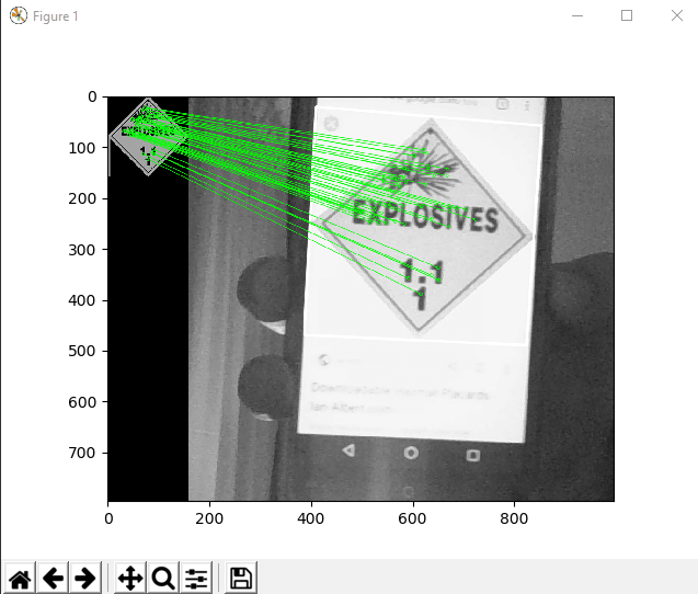
The best matching features have been mapped from a template image to a real-world image (of a hazmat sign on my phone).
Using the following function, we can loop over a series of templates and find the one that best matches an inputted real-world image:
1 2 3 4 5 6 7 8 9 10 11 12 13 14 15 16 | # classify the input image def classify(image, sign_list): # Loop through signs to store bff and color matches for i, sign in enumerate(sign_list): template = cv2.imread(sign.image) sign.bff_data = bff_match(image, template) sign.bff = len(sign.bff_data) # Sort the results using the bff match attribute in reverse order sign_list.sort(key=lambda x: x.bff, reverse=True) best = sign_list[0] best_image = cv2.imread(best.image) return best.name |
In this code, a ‘sign’ class was used to abstract the process of storing information. See ‘classify_abstracted.py’ in SARTVision for the definition of that class, and ‘hazmat.py’ for where the class is used to define a series of templates, which is passed into classify() as the second parameter, sign_list.
The code from this blog post, which is also used by the SART robot, has been taken from the following tutorials, which I strongly recommend as further reading: